September Sampling

Well its been a while since I posted some pictures, so here you go.

This lamprey lost its tail a little while ago and it is slowly growing back. You can see the tip is just a little too small for this animal. He has been marked so I have been able to see its tail grow back slowly.

These two pictures are of the same animal. This is a mayfly (Ephemeroptera), and a burrowing species probably Ephemeridae: Ephemera sp. If you look closely you will see two horns at the front of the head, and if you could have held the animal you would have seen its huge Pop-eye arms. Both of these pieces of its anatomy help it dig. And dig it did, when I released it.

Although it is September already we have not gotten much rain lately. As a result all of these rocks should be covered by water at this time of year, but remain exposed. The lampreys are also quietly waiting for water levels to come up so they can move on to greener pastures.

A shot of the water as it passes over the stream bed.

Its that time of the year, when big ammocoetes become juvenile lamprey and head out to the sea. The silvery lamprey are the bottom are now true juveniles. If they survive the trek to the ocean they will begin their lives their, feeding on other fishes.

Here is a close up of the juveniles (sometimes called transformers or macrophthalmia). One of them was tagged last time, but its body consumed the tag. So it was hard to tell which tag it had. Thankfully, it is a transformer which meant it could only be one animal I saw last time.

A downstream view of the stream, ona rock bar that has been building up slowly all summer.

A picture of the most productive ammocoete area in my study.

Here are a series of pictures of the same animal. It looks like a leaf, but its not a leaf, its a dragonfly. This is Hagenius sp., the common name is dragonhunter (link). This species is a large predatory adult animal that actually actively hunts and consumes other dragonflies. Even though the larvae (pictured here) looks a little weird the adult is a normal looking dragonfly.

Using R to Create Histograms

Histograms are common way to analyze data quickly, and are useful in many studies where time is considered for groups. Excel's anemic histogram options are completely ill suited to scientific needs. However, the R language provides an extremely powerful tool to produce histograms.

In this post I will lead you through ways to modify histograms and produce a range of different plots. If you are new start with the first and word down. Try to understand how each is generated. If you are more familiar with R and the hist() command, scan through the histograms until you find what you are looking for and copy the code.

The data set I use can be found in the package 'fishmethods' and is called Kimura.

Before proceeding and after downloading the package run:

library(fishmethods)
data(Kimura)

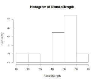
To build a basic histogram select a vector from your dataset. To begin we will use the length data in Kimura.

hist(Kimura$length)

This looks pretty poor at first glace, we need to specify all the pieces we want. We are going to change the text on the axes and the title.

hist(Kimura$length,
     ylab="Counts",
     xlab="Length (cm)",
     main="Pacific Hake")

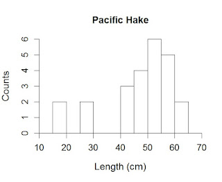
Now we are going to change the bins so that they make more sense for our data. You can either guess at how many breaks you want or you can specify them exactly. If you do not specify the amount of breaks exactly R will make clean breaks. This will cause problems if you are comparing groups because the breaks may not be the same between groups. For many cases it will not matter, but as a matter of course you should specify them exactly. The first code allows R to try to make nice breaks, the second is when I specify them exactly. They produce the same output because I like the breaks R selected.

hist(Kimura$length,
     ylab="Counts",
     xlab="Length (cm)",
     main="Pacific Hake",
     breaks=10)

hist(Kimura$length,
     ylab="Counts",
     xlab="Length (cm)",
     main="Pacific Hake",
     breaks=seq(from=10,to=70,by=5))

Tip: For those familiar with R and know that it is an implicit language you will see inefficiencies in my code. I have explicitly stated components (e.g., the words from and to in seq), this is to help new users. If you are comfortable with the language feel free to clean up the code.

Couple of common complaints now arise, the axes should meet and the text needs to be larger. Let us address both of these issues in the par command. The par command sets the parameters the plot will be drawn in. Changes to these will change how plots are drawn until you either close R again or re-specify.

To make the axes meet at the bottom use the following code:

par(xaxs="i", yaxs="i")
hist(Kimura$length,
     ylab="Counts",
     xlab="Length (cm)",
     main="Pacific Hake",
     breaks=seq(from=10,to=70,by=5))

To change the size of labels and title remain within the par command but write:

par(xaxs="i", yaxs="i", cex.lab=1.2, cex.axis=1.1, cex=1.3)
hist(Kimura$length,
     ylab="Counts",
     xlab="Length (cm)",
     main="Pacific Hake",
     breaks=seq(from=10,to=70,by=5))

The command cex is used to specify sizes of things in a number of plots. cex.lab changes the size of labels on the axes, cex.axis changes the size of the numbers on the axis, and cex changes the size of the title on the plot.

Now we are going to fill in the bars so they are easier to read. There are many ways to do this we can either specify known colors (e.g., "red", "black", "coral", "salmon"), or we can specify the color with numbers related to the value of red, green, or blue component.

par(xaxs="i", yaxs="i", cex.lab=1.2, cex.axis=1.1, cex=1.3)
hist(Kimura$length,
     ylab="Counts",
     xlab="Length (cm)",
     main="Pacific Hake",
     breaks=seq(from=10,to=70,by=5),
     col="salmon")

hist(Kimura$length,
     ylab="Counts",
     xlab="Length (cm)",
     main="Pacific Hake",
     breaks=seq(from=10,to=70,by=5),
     col=rgb(0.5,0.5,0.5))

Things are looking pretty good here, but we should draw box around the plot, again multiple ways to do this.

hist(Kimura$length,
     ylab="Counts",
     xlab="Length (cm)",
     main="Pacific Hake",
     breaks=seq(from=10,to=70,by=5),
     col=rgb(0.5,0.5,0.5))
box()

You can use the above code now with the word box, or you can add axis lines to the open areas where they are normally not plotted.

hist(Kimura$length,
     ylab="Counts",
     xlab="Length (cm)",
     main="Pacific Hake",
     breaks=seq(from=10,to=70,by=5),
     col=rgb(0.5,0.5,0.5))
axis(3, pos=6, labels=F, lwd.ticks=0)
axis(4, pos=70, labels=F, lwd.ticks=0)

Tip: Couple of thoughts here on which to use and why. The box command is simple and easy to use, and I use it whenever I have simple axes I do not care about specifying exactly. It is also useful because you can add more information to it and draw the box in the plot to highlight data. I use the axis command whenever I need to make the axes very specific and when axes might not have the same scale. You can even add multiple axes to a single axis if you have different scales. In short, when you need it simple use box, if you need to specify a different scale use axis.

hist(Kimura$length,
     ylab="Counts",
     xlab="Length (cm)",
     main="Pacific Hake",
     breaks=seq(from=10,to=70,by=5),
     col=rgb(0.5,0.5,0.5),
     axes=F,
     xlim=c(0,80),
     ylim=c(0,10))
axis(1, pos=0, labels=T, at=c(0,20,40,60,80))
axis(2, pos=0, las=1, labels=T, at=c(0,2,4,6,8,10))
axis(3, pos=10, labels=F, lwd.ticks=0)
axis(4, pos=80, labels=F, lwd.ticks=0)

So let us review what we just did. We specified that the axes would not be printed (axes=F), but we set the limits of the axes we knew we wanted (xlim and ylim commands). Then in the axis commands we set where the tick marks would appear (e.g., at=c(0,20,40,60,80)) and for the 3rd and 4th axis we said exactly where they should meet the other axes with the pos command. Using lwd.ticks=0 prevents the tick marks from being drawn.

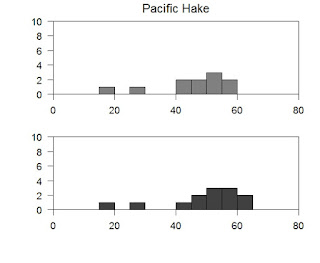
Now we will make multi-panel histograms and then overlapping histograms. Multi-panel histograms are useful if we would like to compare two or more groups simultaneously. In our data set we have only two groups (male or female), but we will write code using a loop in case your data set contains many groups and you want to automate the process instead of specifying everything with hundreds of lines.

First the we will start by specifying exactly what we want.

par(xaxs="i", yaxs="i", cex.lab=1.2, cex.axis=1.1, cex=1.3, mfrow=c(length(unique(Kimura$sex)), 1) )
#########   Our first histogram   ##########
hist(Kimura$length[Kimura$sex=="M"],
     ylab="Counts",
     xlab="Length (cm)",
     main="Pacific Hake",
     breaks=seq(from=10,to=70,by=5),
     col=rgb(0.5,0.5,0.5),
     axes=F,
     xlim=c(0,80),
     ylim=c(0,10))
axis(1, pos=0, labels=T, at=c(0,20,40,60,80))
axis(2, pos=0, las=1, labels=T, at=c(0,2,4,6,8,10))
axis(3, pos=10, labels=F, lwd.ticks=0)
axis(4, pos=80, labels=F, lwd.ticks=0)
 
######### Our second histogram ##########
hist(Kimura$length[Kimura$sex=="F"],
     ylab="Counts",
     xlab="Length (cm)",
     main="Pacific Hake",
     breaks=seq(from=10,to=70,by=5),
     col=rgb(0.25,0.25,0.25),
     axes=F,
     xlim=c(0,80),
     ylim=c(0,10))
axis(1, pos=0, labels=T, at=c(0,20,40,60,80))
axis(2, pos=0, las=1, labels=T, at=c(0,2,4,6,8,10))
axis(3, pos=10, labels=F, lwd.ticks=0)
axis(4, pos=80, labels=F, lwd.ticks=0)

Wow...wait...how did that happen, why is there so much code? Actually, I have simply cut and pasted the code we already used, so while it looks like a lot it is very similar to way we ran. I did make a couple of changes so let us start with the par command.

Here I have inserted the new parameter mfrow. The mfrow parameter specifies how many rows and columns in your image. Since we have two histograms we probably want 2 rows and 1 column. You could also print this as 1 row and two column too. To do so I could have written mfrow=c(2,1). This would be the easiest way to do this, but what if I don't remember how many groups are in my data set or I want R to figure it out on the fly for me. To do this automatically I have R hunt through my sex grouping and pull out all the groups (that is the use of the unique command). This pulls out the values "M" and "F" which are not numbers so cannot tell R how many rows I want. I then use the length command to measure the length of the values (of course it is 2) so it places that value in, and viola it automatically makes 2 rows.

The next change was that I added a rule to what data is plotted. Here the in the hist command you can see I placed brackets after telling R to look at the length column. I then specified which column I want R to look at (Kimura$sex) and then I said only pick values that have a sex column exactly matching (==) the value "M". I copied this and changed it to "F" for the females.

However, after all this work the plots look really poor. They are squished, the data is repeated (Pacific Hake), I don't know which is male or female, and the numbers on the axis overlap. Let us deal with all these problems at once. To do this we return to the par command.

par(xaxs="i", yaxs="i", cex.lab=1.2, cex.axis=1.1, cex=1.3, mfrow=c(length(unique(Kimura$sex)), 1),
    oma=c(3,3,0,0), mar=c(2,2,2,2))
#########   Our first histogram   ##########
hist(Kimura$length[Kimura$sex=="M"],
     ylab="Counts",
     xlab="Length (cm)",
     main="",
     breaks=seq(from=10,to=70,by=5),
     col=rgb(0.5,0.5,0.5),
     axes=F,
     xlim=c(0,80),
     ylim=c(0,10))
axis(1, pos=0, labels=T, at=c(0,20,40,60,80))
axis(2, pos=0, las=1, labels=T, at=c(0,2,4,6,8,10))
axis(3, pos=10, labels=F, lwd.ticks=0)
axis(4, pos=80, labels=F, lwd.ticks=0)
mtext("Pacific Hake", side=1, at=40, line=-8.5, cex=1.4)
 
######### Our second histogram ##########
hist(Kimura$length[Kimura$sex=="F"],
     ylab="Counts",
     xlab="Length (cm)",
     main="",
     breaks=seq(from=10,to=70,by=5),
     col=rgb(0.25,0.25,0.25),
     axes=F,
     xlim=c(0,80),
     ylim=c(0,10))
axis(1, pos=0, labels=T, at=c(0,20,40,60,80))
axis(2, pos=0, las=1, labels=T, at=c(0,2,4,6,8,10))
axis(3, pos=10, labels=F, lwd.ticks=0)
axis(4, pos=80, labels=F, lwd.ticks=0)

To the par command I have added two parameters oma an mar. The oma parameter sets the margins in each plot; position one is side 1, position 2 is side 2, etc. The numbers are the number of lines I would like to see. The oma parameter sets the margins in the window outside of the plots. It follows the same routine as the mar parameter rules.

I have also added a command called mtext, which places text based upon the axis it is called to. Here I have told it to place the words Pacific Hake on the plot following side 1 at 40 (this is based on the x-axis) and then -8.5 (this is based on the y-axis). I also changed the size with cex. Now we have some redundant code floating around so feel free to go in and clean it up.

par(xaxs="i", yaxs="i", cex.lab=1.2, cex.axis=1.1, cex=1.3, mfrow=c(length(unique(Kimura$sex)), 1),
    oma=c(3,3,0,0), mar=c(2,2,2,2))
#########   Our first histogram   ##########
hist(Kimura$length[Kimura$sex=="M"],
     ylab="",
     xlab="",
     main="",
     breaks=seq(from=10,to=70,by=5),
     col=rgb(0.5,0.5,0.5),
     axes=F,
     xlim=c(0,80),
     ylim=c(0,10))
axis(1, pos=0, labels=T, at=c(0,20,40,60,80))
axis(2, pos=0, las=1, labels=T, at=c(0,2,4,6,8,10))
mtext("Counts", side=2, at=5, line=2.5, cex=1.3)
axis(3, pos=10, labels=F, lwd.ticks=0)
axis(4, pos=80, labels=F, lwd.ticks=0)
mtext("Pacific Hake", side=1, at=40, line=-8.5, cex=1.4)
 
######### Our second histogram ##########
hist(Kimura$length[Kimura$sex=="F"],
     ylab="",
     xlab="",
     main="",
     breaks=seq(from=10,to=70,by=5),
     col=rgb(0.25,0.25,0.25),
     axes=F,
     xlim=c(0,80),
     ylim=c(0,10))
axis(1, pos=0, labels=T, at=c(0,20,40,60,80))
mtext("Length (cm)", side=1, at=40, line=2.5, cex=1.3)
axis(2, pos=0, las=1, labels=T, at=c(0,2,4,6,8,10), ylab="Counts")
mtext("Counts", side=2, at=5, line=2.5, cex=1.3)
axis(3, pos=10, labels=F, lwd.ticks=0)
axis(4, pos=80, labels=F, lwd.ticks=0)

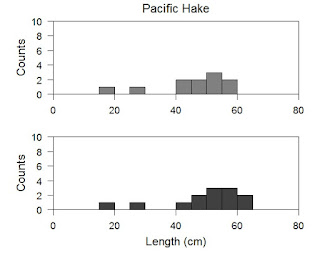
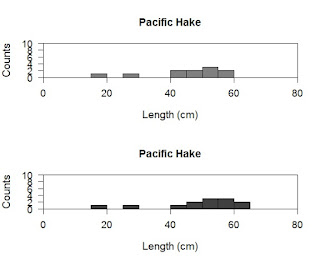
Alright here I have used mtext to add the labels back to the axes again. If you want to label your plots you could also have mtext draw "(a)" and "(b)" to designate which plot is which. I am going to pretty up this plot in the final step and then we are going to move onto a loop to do all this automatically.

par(xaxs="i", yaxs="i", cex.lab=1.2, cex.axis=1.1, cex=1.3, mfrow=c(length(unique(Kimura$sex)), 1),
    oma=c(5,3,2,2), mar=c(0,2,0,0))
#########   Our first histogram   ##########
hist(Kimura$length[Kimura$sex=="M"],
     ylab="",
     xlab="",
     main="",
     breaks=seq(from=10,to=70,by=5),
     col=rgb(0.5,0.5,0.5),
     axes=F,
     xlim=c(0,80),
     ylim=c(0,10))
axis(1, pos=0, labels=F, at=c(0,20,40,60,80))
mtext("\u2642", side=1, at=70, line=-7.5, cex=2)
axis(2, pos=0, las=1, labels=T, at=c(0,2,4,6,8,10))
mtext("Counts", side=2, at=5, line=2.5, cex=1.3)
axis(3, pos=10, labels=F, lwd.ticks=0)
axis(4, pos=80, labels=F, lwd.ticks=0)
mtext("Pacific Hake", side=1, at=40, line=-10.5, cex=1.4)
 
######### Our second histogram ##########
hist(Kimura$length[Kimura$sex=="F"],
     ylab="",
     xlab="",
     main="",
     breaks=seq(from=10,to=70,by=5),
     col=rgb(0.25,0.25,0.25),
     axes=F,
     xlim=c(0,80),
     ylim=c(0,10))
axis(1, pos=0, labels=T, at=c(0,20,40,60,80))
mtext("\u2640", side=1, at=70, line=-7.5, cex=2)
mtext("Length (cm)", side=1, at=40, line=2.5, cex=1.3)
axis(2, pos=0, las=1, labels=T, at=c(0,2,4,6,8,10), ylab="Counts")
mtext("Counts", side=2, at=5, line=2.5, cex=1.3)
axis(3, pos=10, labels=F, lwd.ticks=0)
axis(4, pos=80, labels=F, lwd.ticks=0)

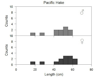
I added the male and female symbols with unicode text, again with the mtext command. You can, and should, feel free to change colors as you see fit. Of course you can test yourself by trying the traditional blue and pink for boys and girls, but do not arbitrary gender colors limit your creativity. Also you should, at this point, feel in control of many other parts of the plot and should experiment as you see fit.

Now our code is starting to get a little ugly, it is very long. As the length of the code increases it becomes increasingly more difficult to identify and correct errors. The simplest code is the best code is a good principle to live by. In the next plot we are going to use a loop to do the hard work for us. If you know nothing about loops its ok to end here. If you want to use loops to automate your own work though do push on.

#Make a new column to help us in the next step
Kimura$sex_v <- as.numeric(Kimura$sex)
 
#Now make the plots
par(xaxs="i", yaxs="i", cex.lab=1.2, cex.axis=1.1, cex=1.3, mfrow=c(length(unique(Kimura$sex)), 1),
    oma=c(5,3,2,2), mar=c(0,2,0,0))
for ( i in 1:length(unique(Kimura$sex)) ) {
  hist(Kimura$length[Kimura$sex_v==i],
       ylab="",
       xlab="",
       main="",
       breaks=seq(from=10,to=70,by=5),
       col=rgb(i/4+0.25,i/4+0.25,i/4+0.25),
       axes=F,
       xlim=c(0,80),
       ylim=c(0,10))
  axis(1, pos=0, labels=F, at=c(0,20,40,60,80))
 
  axis(2, pos=0, las=1, labels=T, at=c(0,2,4,6,8,10))
  mtext("Counts", side=2, at=5, line=2.5, cex=1.3)
  axis(3, pos=10, labels=F, lwd.ticks=0)
  axis(4, pos=80, labels=F, lwd.ticks=0)
}
axis(1, pos=0, labels=T, at=c(0,20,40,60,80))
mtext("Length (cm)", side=1, at=40, line=2.5, cex=1.3)
 
mtext("Pacific Hake", side=1, at=40, line=-19.5, cex=1.4)
mtext("\u2642", side=1, at=70, line=-16.5, cex=2)
mtext("\u2640", side=1, at=70, line=-7.5, cex=2)

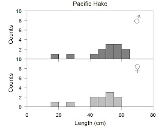
The loop has reduced our lines considerably. Technically a loop is a single line and can be collapsed in programs like Rstudio (which you should be using anyway) to help neaten up your work when you do not need it. You can see how I manipulated the loop by calling upon i, which R will understand to be a number, and placed it wherever I wanted to change things. The loop does repeat the same operation over and over again so if you copied our exact code down you would find that we have labels printed incorrectly. Carefully go through my code and see how I get to this. As a side note, good practise would be to go through this code and eliminate unnecessary pieces. You can also experiment with if/then statements in the loop to get finer control within it. See if you can further reduce the number of lines.

Tip: Efficiency is nice, but time is money. I reduce my code based upon my own experience of what I know well and what would be easy to do. There are more efficient ways for sure, but these require my time. As a result, I often have less efficient code than I could develop, but I find that few people care because they only see the results anyway.

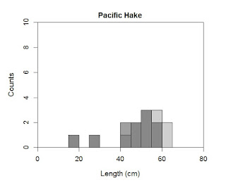
Finally, let us produce stacked histograms. I rarely recommend these, but they can be useful in limited cases. Be careful though because their ease of production does not always mirror their ease of readability. All we need to do to get these is tell R that instead of making a new plot, it is to add our second plot to the first. We need to specify par again or we are going to have some problems.

par(xaxs="i", yaxs="i", cex.lab=1.2, cex.axis=1.1, cex=1.3, mfrow=c(1, 1),
    oma=c(1,1,1,1), mar=c(4,4,2,2))
hist(Kimura$length[Kimura$sex=="M"],
     ylab="Counts",
     xlab="Length (cm)",
     main="Pacific Hake",
     breaks=seq(from=10,to=70,by=5),
     col=rgb(0.5,0.5,0.5,0.75),
     axes=T,
     xlim=c(0,80),
     ylim=c(0,10))
hist(Kimura$length[Kimura$sex=="F"],
     breaks=seq(from=10,to=70,by=5),
     col=rgb(0.25,0.25,0.25,0.25),
     add=T)
box()

The rgb parameter now includes a fourth value. This value specifies the transparency you wish to apply. Zero would provide a fully transparent overlay, and 1 would make the color overwrite (i.e., there would be no transparency). I have also added in the second hist command the parameter add=T. This tells R to place the new plot on the old plot. You can also change the number of breaks in each plot separately (I can think of no case in which this would be a good idea).

Another overlapping histogram example is located at the link. In their example they use a random number generator (command rnorm) to make up their data. You can experiment with it, otherwise they lead you through the process identically. You will also find lots of interesting R materials at the site.

That is all for now, happy R'ing.